


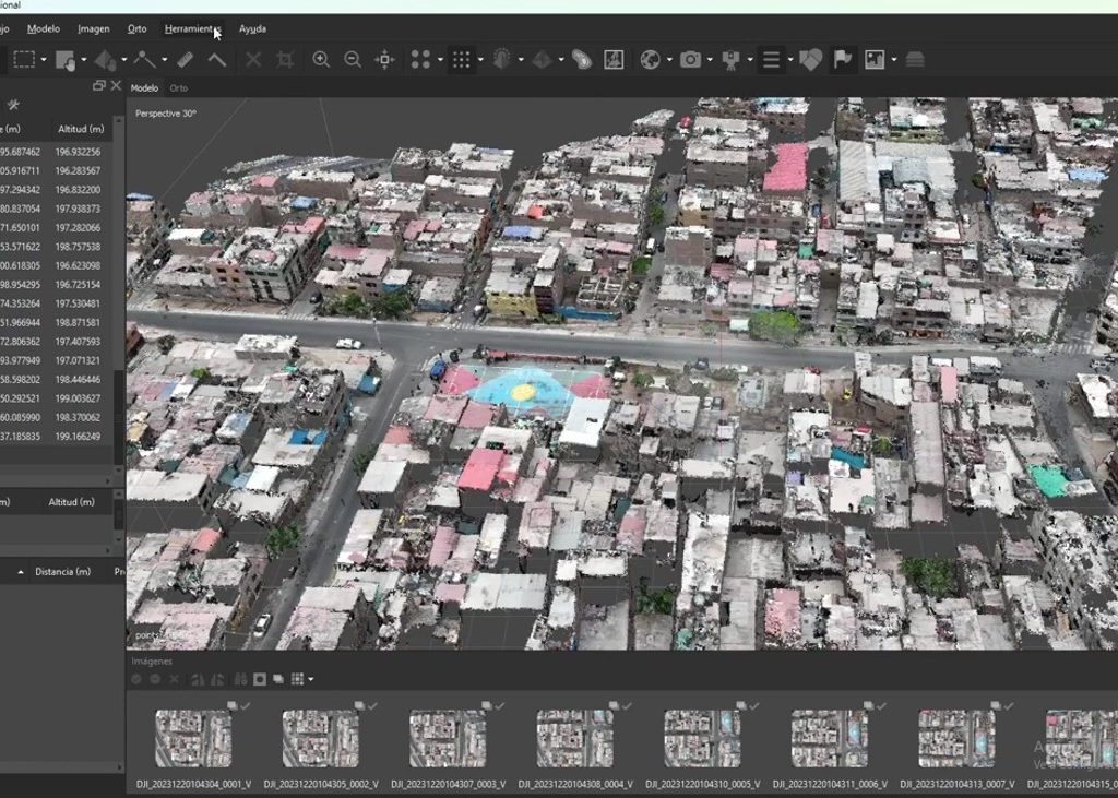
The dense point cloud is the heart of the photogrammetric workflow in Agisoft Metashape. It’s the product from which almost everything else is derived: the 3D mesh, the digital elevation model, the orthomosaic, and the volumetric measurements. Processing it correctly—by choosing the right parameters, editing the result, and exporting in the correct format—makes the difference between an accurate model and one full of noise and gaps. This guide walks you through each stage of the process.
What is a dense point cloud?
A dense point cloud is a collection of millions of three-dimensional points, each with XYZ coordinates and RGB color values, representing the geometry of the photographed scene. It is generated from the depth maps that Metashape calculates for each image once the cameras are aligned.
Unlike the sparse point cloud generated in the alignment stage (with tens of thousands of points), the dense cloud can contain from hundreds of thousands to hundreds of millions of points, depending on the quantity and resolution of the images and the quality parameters chosen.
Step 1: Make sure you have the cameras properly aligned
A dense point cloud can only be generated after the photos have been aligned. If the cameras are not properly aligned, the dense point cloud will reflect those errors in an amplified way: gaps, double surfaces, excessive noise.
Before proceeding, check these indicators in the sparse cloud:
- Reprojection error: should be less than 1 pixel . You can see it in the processing report ( Tools → Processing Report ).
- Camera alignment coverage: At least 90% of imported photos should be aligned. If the percentage is lower, check image quality and overlap.
- Camera distribution: In the 3D view, the camera positions must form the expected trajectory without any “loose” cameras or cameras too far from the group.
If the reprojection error is greater than 1 pixel, optimize the cameras before continuing: Tools → Optimize Cameras . Enable the parameters f, cx, cy, k1, k2, k3, and p1, p2 for better results.
📷 Image Idea (IA): 3D view of a scattered point cloud with camera positions represented as small icons forming a U-shaped path over an object, technical visualization style on a dark background.
Step 2: Generate the dense point cloud
With the cameras aligned, go to:
Workflow → Build dense point cloud
The configuration dialog opens with the following main parameters:
Quality
Quality determines the resolution at which images are processed to calculate depth maps.
| Quality | Processing resolution | Estimated time* | When to use it |
|---|---|---|---|
| Ultra High | Original resolution (1:1) | Very long | Small objects, maximum detail, cultural heritage |
| High | Half the resolution (1:2) | Long | Standard professional projects, surveying |
| Average | One-quarter of the resolution (1:4) | Moderate | Large projects, first review |
| Low | One eighth of the resolution (1:8) | Short | For rapid testing only |
| Lower | One sixteenth (1:16) | Very short | Diagnosis only |
*Time varies considerably depending on the hardware, especially the available GPU and RAM.
Practical recommendation: For most professional projects, High is the optimal balance between quality and processing time. Ultra High is only justified when millimeter detail is critical or when the object is small and there are few images.
Depth filtering
Controls how inconsistent or noisy points are handled during generation.
| Filtered | When to use it |
|---|---|
| Mild | Complex surfaces, vegetation, irregular objects. Preserves more points, including fine edges. |
| Moderate | General use. Good balance between density and cleanliness. |
| Aggressive | Smooth, regular surfaces such as interiors, tracks, or open terrain. Removes more noise but may lose fine details. |
Calculate the confidence level of the point
Enabling this option ( Calculate point confidence ) assigns each point a confidence value (0–255) indicating how reliable its calculated position is. This is very useful if you plan to filter out low-quality points after processing. It is recommended to always enable this option.
📷 Image Idea (AI): Stylized capture of Metashape’s “Build Dense Point Cloud” settings dialog, with parameters visible, on a dark interface background.
Step 3: Evaluate the generated point cloud
Once the processing is complete, before moving on to the next stage, examine the dense cloud:
What to look for:
- Full coverage: the entire area of interest must be represented without significant gaps.
- Uniform density: the density of points should be homogeneous. Lighter or scattered areas indicate overlap problems or problematic surfaces.
- Absence of obvious artifacts: floating points, duplicate surfaces, or “ghosts” of moving objects.
If you encounter serious coverage problems, the most effective solution is to add more photos of the deficient areas and reprocess them. If the problem is noise, manual editing (next step) can resolve it.
📷 Image idea (AI): Dense point cloud of a historic building or bridge, millions of points with RGB color gradient on a black background, scientific visualization style.
Step 4: Edit the point cloud (cleaning)
Metashape offers tools to manually edit the dense point cloud and remove unwanted points before generating derivative products.
Manual selection
Use the selection tools in the toolbar:
- Rectangle / Lasso / Polygon: select points within an area drawn in the 3D view.
- Free selection: allows you to draw an irregular selection region.
Once you’ve selected the items to delete, press Delete to erase them. This is ideal for removing:
- Points on the ground that are not part of the object of interest
- Vegetation surrounding a structure
- Points generated by moving objects (people, vehicles)
- Point clouds of areas outside the work area
Tip: Before editing, duplicate the chunk ( right-click on the chunk → Duplicate chunk ). This way you can revert the changes if something goes wrong, without having to reprocess.
Filtered by trust
If you activated “Calculate point confidence” in the previous step, you can quickly filter out the least reliable points:
Tools → Dense Point Cloud → Filter by Trust
Adjust the minimum confidence threshold (e.g., remove all points with less than 2 confidence) to automatically clean up noise without manual point-by-point intervention.
📷 Image idea (AI): Side-by-side comparison: left point cloud with noise and floating points, right the same cloud clean and uniform, dark background, technical style.
Step 5: Classify the point cloud (Professional only)
Classification is one of Metashape Professional’s most powerful features. It allows you to assign a semantic category to each point, so that derived products (especially DEM/DTM) can be generated only from relevant points.
Tools → Dense Point Cloud → Classify Ground Points
Available point types
| Class | Description |
|---|---|
| Ground | Bare ground points |
| Low vegetation | Lawn, low shrubs |
| Medium vegetation | Medium-height shrubs |
| Tall vegetation | Trees |
| Buildings | Built structures |
| Unclassified | Points not assigned to any class |
Terrain classification parameters
| Parameter | Description |
|---|---|
| Maximum angle | Maximum slope of the terrain (in degrees). Increasing this value allows for the classification of steeper areas as terrain. |
| Maximum distance | Maximum distance between points on the terrain and the estimated area |
| Cell size | Analysis grid resolution. Lower values = more accuracy, more time |
After automatic classification, you can manually refine using the selection tools to reclassify individual points or specific regions.
The classification of terrain points is essential to generate a DTM (Digital Terrain Model) that represents only the ground without vegetation or buildings, unlike the DSM (Digital Surface Model) which includes everything.
📷 Image idea (AI): Point cloud classified with colors by class: brown for terrain, green for vegetation, gray for buildings, on a black background, professional GIS style.
Step 6: Export the point cloud
With the cloud processed, edited, and classified, the final step is to export it to the appropriate format for the target software.
File → Export → Export point cloud
Available export formats
| Format | Extension | When to use it |
|---|---|---|
| THE | .las | Industry standard for geospatial point clouds. Compatible with ArcGIS, QGIS, CloudCompare, and AutoCAD Civil 3D. |
| LAZ | .laz | Compressed version of LAS. Same content, up to 10x less disk space |
| PLY | .ply | For use in 3D software (Blender, MeshLab) |
| XYZ / TXT | .txt | Simple text format, coordinates separated by spaces or commas. Compatible with almost everything. |
| PTS | .pts | Compatible with laser scanning software (Leica Cyclone, etc.) |
| E57 | .e57 | Standard for 3D scan data, compatible with BIM and surveying software |
Important export options
Coordinate system: If the project is georeferenced (with GCPs or GPS), choose the correct reference system for the destination. In Argentina, the most common are WGS84, POSGAR 07, or the corresponding Gauss-Krüger projections.
Save colors: Activate this option to preserve the RGB values of each point, essential for visualization.
Save point classes: If you classified the cloud, activate this option so that the classes are saved in the exported LAS/LAZ file and are recognizable by the destination software.
Save trust: export the trust value as an additional attribute of each point.
Common mistakes and how to fix them
The dense cloud has many gaps. Most frequent cause: insufficient overlap between images. It can also be due to surfaces without texture (water, glass, polished metal) or areas photographed from a single angle. Solution: add complementary photos of the problem areas and reprocess.
The cloud has too much noise or floaters. Cause: low-quality images, movement during capture, reflections, or underlit areas. Solution: use Moderate or Aggressive depth filtering, filter by trust, and manually clean up with selection tools.
Processing is very slow or the computer runs out of memory. Cause: The project is too large for the available hardware or the quality setting is too high. Solution: Reduce the quality to Medium, divide the project into smaller chunks, or add more RAM to the computer.
Terrain classification does not work well in areas with dense vegetation. Cause: In forests or areas with very dense vegetation cover, few laser (or photogrammetric) beams reach the actual ground. Solution: Adjust the maximum angle and cell size, and supplement with manual classification in problem areas.
The exported points do not have correct coordinates. Cause: The project was not georeferenced with GCPs, or the export coordinate system does not match the expected one. Solution: Verify that the GCPs are correctly marked and that the coordinate system in the Reference panel is correct before exporting.
Conclusion
Processing a point cloud correctly in Metashape is more than just pressing a button. Choosing the right quality for the project, cleaning up problematic points, classifying terrain for GIS projects, and exporting in the correct format are all decisions that directly impact the quality of all resulting products.
If you’re starting out with photogrammetry or evaluating whether Agisoft Metashape fits your workflow, at Aufiero Informática we can advise you without obligation.
👉 View Agisoft Metashape licenses at Aufiero Informática
Frequently Asked Questions
How long does it take to generate a dense point cloud? It depends on the hardware and settings. For reference, 300 photos at 20 MP in High quality with an RTX 4070 GPU takes approximately 45–90 minutes. In Ultra High quality, that time can triple.
Can I generate a dense cloud without a GPU? Yes, but the speed difference is very significant. The GPU accelerates the calculation of depth maps, which is the most intensive operation at this stage. Without a dedicated GPU, medium-sized projects can take many hours.
Does dense point cloud technology replace LiDAR scanning? For many applications, yes, especially when data isn’t needed under dense vegetation. Photogrammetry generates textured point clouds (RGB color per point), which LiDAR doesn’t do by default. For forest canopy penetration, however, LiDAR remains superior.
Can I edit the dense point cloud after generating the mesh? Yes, the point cloud and the mesh are separate products. You can edit the point cloud and regenerate the mesh without having to re-align the photos.
What is the difference between DSM and DTM? The DSM (Digital Surface Model) includes all objects on the ground: buildings, vegetation, infrastructure. The DTM (Digital Terrain Model) represents only the bare ground and is generated from points classified as “terrain” in the point cloud.